From Zero to Banned: Make Othello AI at home

This project took longer than expected—but finally, here’s a quick walkthrough of how to built OthelloZero agent. The code is available here.
Intro
I genuinely wanted to train something using the pure Zero approach. The target environment didn’t need to be overly complex, but it also shouldn’t be trivial. The classic 8x8 Othello board struck a nice balance—it’s rich in strategy, yet simple enough to do fast experiments. Even better, there were existing online benchmarks available: strong, publicly accessible bots and competitive platforms with human opponents. This meant I wouldn’t need to build my own benchmarks to measure progress—an already promising start.
Originally, I planned to finish this project in a month. It ended up taking four with the full-time work, travelling, procrastination, etc. Overall, I am happy with the outcome: without spending much money, I managed to train a strong bot that competes on par with some of the best human players (I do not dare to make a stronger statement due to the lack of proper evaluation). All done via a pure Zero training pipeline.
As a bit of a stress test, I played my smaller model version on the Othello Quest app, going up against top-rated human players. Over five days, the bot maintained a strong win rate (with only ~5 losses), climbed to 2250 ELO, and secured 49th place out of ~45k players—until I got banned (sorry to anyone impacted). While I don’t encourage unfair play, this made the project much more fun.
Beyond that, the smaller model managed to be on par with the Egaroucid bot at level 8, and my larger model (more parameters) beat it at level 10 (this, with high probabillity, would be a superhuman level).
Key Milestones Achieved:
- Beating MCTS with random rollouts.
- Beating MCTS guided by a supervised policy trained on data from top human players.
- Small model defeating many top players on Othello Quest, achieving 2250 ELO and 49th place out of ~45k.
- Large model beating Egaroucid at level 10.
Benchmarks
To effectively track progress in training an Othello-playing agent, I established three clear benchmarks: a superhuman bot, a supervised model trained on expert human gameplay and playing against top-humal players on Othello Quest platform.
Egaroucid
Egaroucid is among the strongest available Othello bots. It offers an accessible web interface and was straightforward to install on macOS. Egaroucid has 60 difficulty levels, with higher levels performing deeper minimax searches. Although there isn’t a definitive reference, it’s reasonable to consider level 10 (a 10-move lookahead mid-game) as superhuman, given top human cognitive capabilities peak around an 8–10 move lookahead. By regularly evaluating our agent against Egaroucid at this level, we can reliably measure our progress toward surpassing human expertise.
Supervised Model
To approximate human-level performance in Othello, I employed a supervised learning approach using a dataset consisting of ~ 25k games recorded from the top 100 players on eOthello. Each game has around 60 moves, providing extensive data for model training. Establishing a supervised learning baseline helps set a clear target to exceed, and it enables faster iteration and selection of model architectures before beginning reinforcement learning experiments, which are comparatively slower. The dataset provides explicit labels: the ground truth for the value function corresponds to the final game outcome, while the ground truth for the policy function is a one-hot encoded vector indicating the player’s move. Our objective is to mimic these expert players with our model.
Similar to AlphaZero, our model architecture features a single backbone with two distinct heads: one for policy estimation and one for value prediction. The combined loss function includes a cross-entropy loss for the policy head and a mean squared error (MSE) loss for the value head. To better represent the significance of mid-to-late game positions, moves from earlier stages of games were sampled less frequently: 30% of moves are sampled from plies less than 8, 70% from plies less than 16, and the rest remain unchanged. Additionally, when multiple players took different actions from the same state, a majority voting scheme was employed.
Furthermore, data augmentation using random dihedral-8 symmetries was applied to reduce overfitting and improve generalization. The dataset was split into train and test sets by game, and the primary evaluation metric was the model’s accuracy in predicting the actual moves made by human experts. With the current setup—a model featuring 128 filters and 5 ResNet blocks (similar architecture to AlphaZero)—I achieved roughly a 59% accuracy. Scaling the model size beyond this configuration did not lead to further improvements, making this model the established baseline for my experiments.
Othello Quest
To benchmark our model against top human players, I registered on the Othello Quest platform and manually played games against skilled opponents. This provided a valuable baseline to assess our model’s strength relative to human expertise.
Training recipe
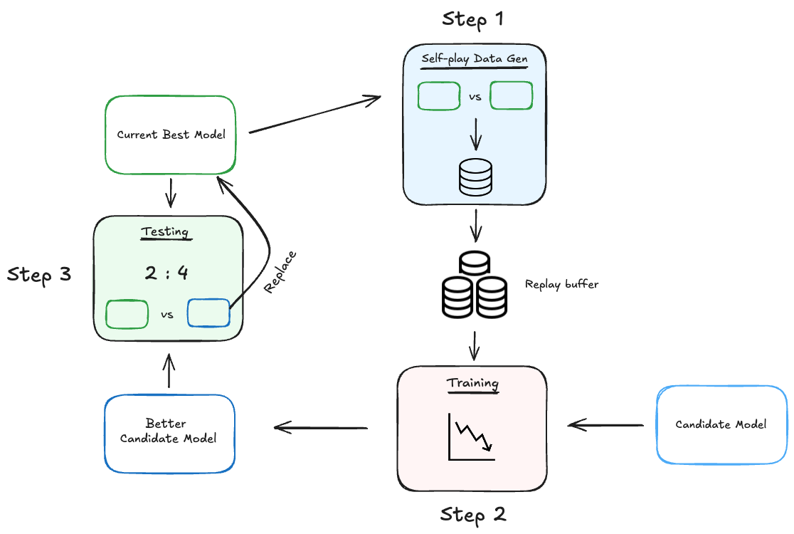
Figure: Overall Training Pipeline
The complete training pipeline is illustrated above and closely follows the methodology outlined in the original AlphaZeroGo paper and my previous blog post.
For clarity, my pipeline employs two primary models:
- Small model (~600k parameters)
- Big model (~1.5M parameters, similar to the original AlphaZero architecture with 5 ResNet blocks and 128 filters, same as in
Supervised Modelsection)
Initially, training starts with a randomly initialized Small model.
1. Data Collection
The model generates training data through self-play, where it competes against itself using Monte Carlo Tree Search (MCTS) for policy improvement. The resulting games are stored in a replay buffer for training.
2. Training
The collected data is used to train the model for a predetermined number of epochs, applying an entropy regularization term to stabilize policy learning.
3. Evaluation
After training, the updated model plays 50 games against the current best model (the data-collection model). If the new model wins more than 60% of these matches, it replaces the previous best model. This gating mechanism prevents drifting into poor local minima, enhances stability, and provides clear tracking of performance gains. Although it slightly slows the pipeline, it greatly facilitates debugging and confidence in the training process.
Details
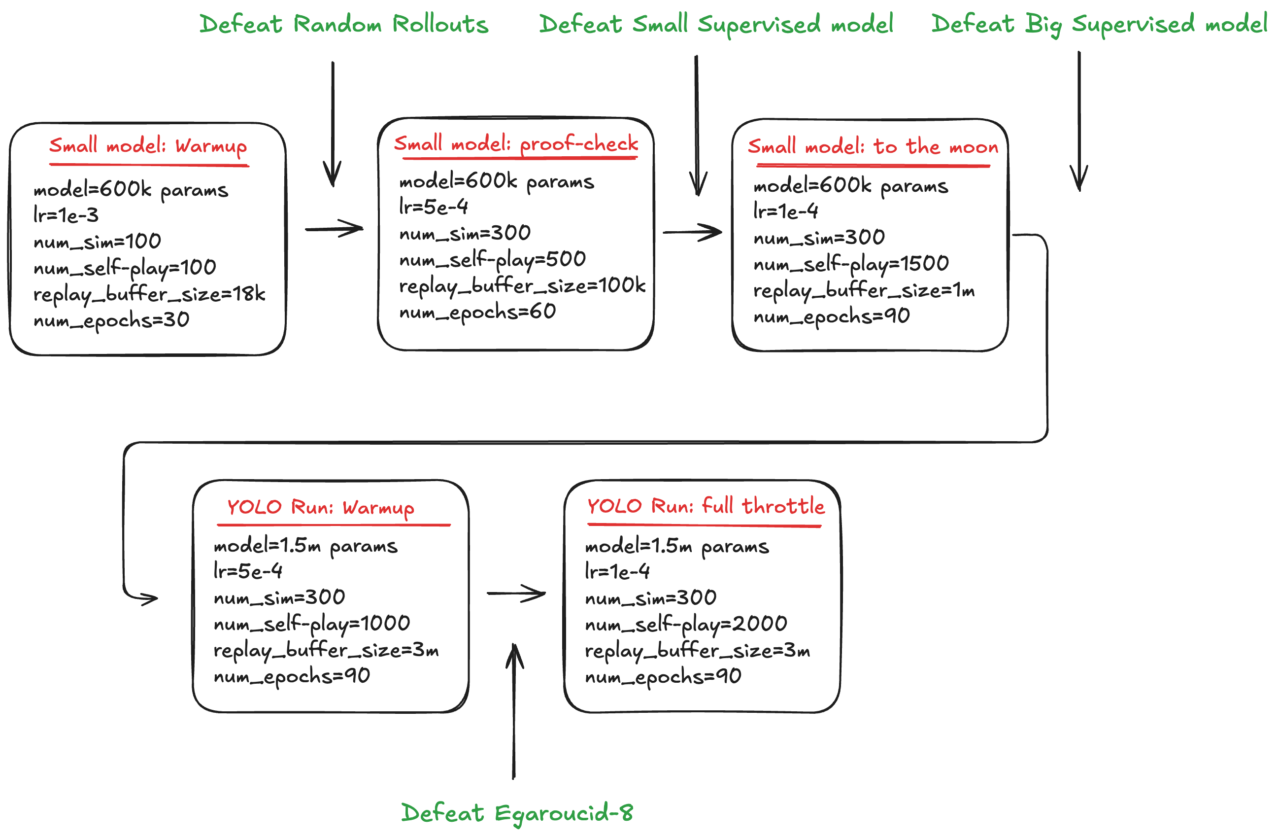
Figure: Training Parameters Schedule
To optimize training efficiency, the pipeline starts with the Small model (600k parameters), which offers quicker iteration for all: self-play, training, and evaluation phases. Once the Small model achieves sufficient performance, I reuse both this trained Small model and its replay buffer as a starting point for training the Big model. This significantly improves convergence, preventing the Big model from starting from scratch and wandering aimlessly.
The training progression involves four main phases:
-
Small Model Warm-up:
Train the small, randomly initialized model until it reliably surpasses an MCTS baseline with random rollouts (beats > 95% of the time). -
Small Model proof check:
Increase the parameters to moderate sizes and confirm continuous performance gains. The objective is to train until this model consistently beats (100% of the time) the supervised Small model (identical architecture). -
Full Throttle (Small Model):
Further train the small model until it outperforms (beats 100% of the time) the supervised Big model benchmark, indicating a robust baseline. -
YOLO run:
Use Small model as a first data-collection model and reuse its replay buffer. The larger model quickly learns to surpass the smaller model, then continues to improve independently. Do it until you run out of money. Adjust hyperparameters whenever we beat Egaroucid-8.
Input representation for the network: in my case to not complexify things I chose to use a canonical board representation (player * board_state) for the input, there is no need in any past information in the input since in Othello the game state is fully observable from the board position.
Augmentations
During training, I apply random dihedral-8 symmetry augmentations to the input state variable before passing it to the model. This imporves resuls for both augmentation supervised and reinforcement learning runs. Is it still Zero approach after that?
Deciding on the number of simulations
To determine a suitable number of simulations per move during training, I followed a simple idea: when using MCTS with random rollouts, the value predictions between consecutive steps should not fluctuate significantly. If increasing the number of simulations no longer provides a noticeable reduction in the variance of the value estimates, I treat that as a good stopping point for the number of simulations.
Empirically, it was found that around 300 simulations were (qualitatively) enough to stabilize significantly the value function. Beyond this point, additional simulations did not drastically reduce the variance in value predictions. This made 300 a reasonable choice for the MCTS simulation count during self-play training.
Evaluation
Here I present the evaluation results against three benchmarks mentioned above.
-
Comparison with Egaroucid:
The Small model performed comparably to Egaroucid at difficulty level 8, achieving a balanced result over 50 games: 23 wins, 23 losses, and 4 draws, at 1200 simulations per move. The Big model played 50 games with Egaroucid-10: 23 wins, 18 losses, 9 draws. -
Comparison with the supervised model:
During training, even the Small Zero model successfully outperformed the Big supervised model. This assessment used 400 simulations per move, but increasing to 800 simulations did not alter the model ranking. -
Comparison with human players:
To verify if the model reached expert human performance, I manually played approximately 60 games on Othello Quest, using the model with 800 simulations per move. I reached a rating of 2250, placing me 49th among ~45k players before getting banned (it would’ve been a better story if I had made it to the top spot—but this is life). During these games, I lost about 5 matches, and my strongest opponent defeated had a rating of 2355.
C_puct parameter seems to significantly affect inference performance. I found that setting c_puct = 3 provided the best results (c_puct = 2 was used during training). Here is the intuition for this parameter: setting it too low results in insufficient short-term exploration (rely more on the value function), while setting it too high reduces the effective depth (long-term planning capacity) of the MCTS algorithm (rely more on the local exploration).
Augmentations during inference: Similar to AlphaZero, applying random dihedral-8 symmetry augmentations during MCTS simulations—before neural network evaluation—provided improved inference stability. This procedure averages out model biases, leading to more robust value predictions.
Learnings from experiments
More Simulations vs. More Games
Balancing compute between conducting extensive simulations per move and generating more games to expand the training dataset involves a key trade-off:
- More simulations per move: Produces stronger policy targets but results in fewer games, and thus fewer unique states in the replay buffer.
- More games with fewer simulations: Yields more data (more states), but potentially weaker policy targets.
My strategy was to increase the number of simulations—from small 100 to a moderate 300—as the model improved (e.g., once it started outperforming MCTS with random rollouts). Overall, I focused on generating more games to ensure the training pipeline was exposed to a wider range of states. This helps to prevent divergence into regions of the state space where the model has no reliable estimates when playing against humans or bots.
Ground truth noise
In the beginning, the model was very hard to train—it couldn’t consistently beat the MCTS baseline with random rollouts. Assuming there were no bugs in the code, I narrowed the potential causes down to two main factors: model capacity and data quality. Increasing model capacity is expensive and time-consuming to test. Besides, the baseline it was failing to beat was weak enough that a ~600K parameter model should be able to outperform it. The first issue I identified was that the replay buffer was too small. Increasing its size helped the model beat MCTS with random rollouts, but convergence toward beating the small supervised model remained slow. My primary suspicion was on the value function ground truths. It’s quite intuitive: from a given state—especially early in the game—different sequences of actions can lead to different outcomes (win/loss) depending on the level of the player. Therefore, the same state can have widely varying value labels, resulting in noisy training targets.
Indeed, by plotting the variance of value ground truths across many states, I observed variances close to 1 in several cases. This high variance may confuse the model and slower the convergence.
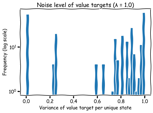
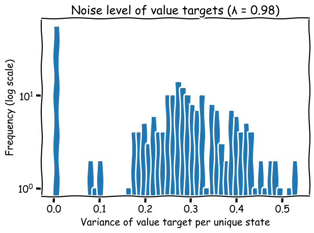
Figure: Noise level of value targets
Smoothing Value Estimates with Lambda-Returns
To address this, I implemented the λ-return technique—partly because it’s an elegant idea I had always wanted to use, and partly because it was well-suited to our setup. I reused value statistics gathered during MCTS simulations to compute lambda-returns.
There are two main reasons to use this approach:
- Variance reduction: Lambda-returns smooth out high-variance Monte Carlo targets by incorporating value estimates along the trajectory.
- Reliable late-game targets: In our case, each MCTS value is derived from many simulations (instead of just one - the game outcome (GO)). For late-game states, these often approximate unbiased Monte Carlo estimates. Thus, for those states, the value targets are based on aggregated outcomes of many random simulations rather than a single rollout. These high-quality targets can then propagate backward (greed arrows below), improving the accuracy of value estimates in mid-game states (yellow arrows). In the illustration below, the upper part shows a tree of simulations, where many of the late-game states simulations result in the true game outcome (GO) (green arrows). This reduces bias in value estimation. By averaging the true outcome (GO) (below) with these simulated estimates, the resulting signal becomes more informative. This also helps to improve estimation of the mid-game states (yellow arrows), while initial states are mainy estimated with bootstrapping (red arrows).
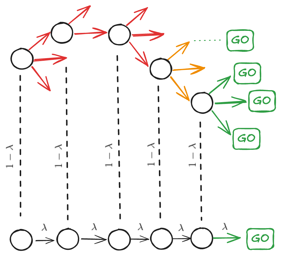
Figure: lambda-return with the tree
Our game has 60 turns, so I selected λ = 0.98 to stay close to the less-biased Monte Carlo estimate (avoiding excessive bootstrapping). For mid-game states, this results in approximately a 0.5 weight on the MC estimate, which seemed like a reasonable compromise.
At each time-step, Monte-Carlo evaluation updates the value of the current state towards the return. However, this return depends on the action and state transitions that were sampled in every subsequent state, which may be a very noisy signal. In general, Monte-Carlo provides an unbiased, but high variance estimate of the true value function \(V^{\pi}(s)\). — Silver, PhD Thesis
Averaging Duplicated Targets
Another noise-reduction technique I used was to average the value and policy targets for repeated (state, model) pairs in the replay buffer. This is especially helpful for early-game states, which are overrepresented due to the structure of self-play. Averaging these duplicates reduces noise and implicitly strengthens the target policy, since it’s akin to simulating more rollouts from the same state.
Simulation Budget and Exploration-Variance Trade-offs
It’s important to recognize that value target variance also depends on how many tree simulations are performed and the amount of exploration in self-play. Due to compute and time constraints, it was limited to 300 simulations per move. I suspect that with deeper searches (e.g., 800 simulations), MCTS would more consistently pick the same optimal actions for a given state, reducing target variance. Exploration parameters also play a major role. Increasing the temperature or Dirichlet noise promotes exploration but increases label noise. Reducing them lowers variance but risks the model getting stuck in local optima. My strategy was to keep exploration relatively high throughout training and address the resulting noise in the training pipeline (λ-return, Averaging Duplicates)—not during data collection.
Rock-paper-scissors trap
If exploration during self-play is too low, the trained policy can become overly specialized, mastering only a narrow subset of states. During evaluation, it might consistently beat the previous greedy policy and get promoted, only to lose subsequently to older policies—creating a cyclical “Rock-Paper-Scissors” scenario.
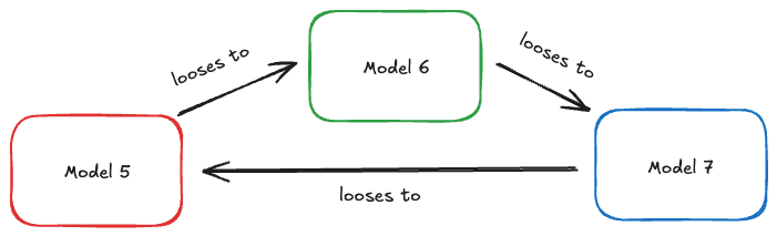
Figure: Rock-Paper-Scissors trap illustration
Initially, I discarded older training data whenever updating the policy to prevent off-policy bias. However, this led to the model forgetting previously learned patterns and exhibiting the cyclic behavior described above. Introducing a replay buffer with a large number of past games helped to mitigate this effect. Still, through careful analysis—particularly by regularly comparing trained models against a stable supervised benchmark—I observed periodic performance oscillations. Newer versions of the model would sometimes lose completely to the supervised model, while earlier versions had been able to beat it.
By testing the model in a wild (against Egaroucid bot and people), I found that the policy had become overly peaked, leading to insufficient exploration—often visiting only one child node in MCTS. Overly peaked policies (i.e., high bias) limit the effectiveness of increasing MCTS simulations, because depth (focused exploration) dominates breadth (general exploration). From previous post we know that given enough simulations, UCT can identify the best move—there is no bias there, or, in simple terms, the policy prior is uniform. However, in my case, the problem was that the policy prior was so peaked that alternative actions were rarely explored. This made the policy brittle and unable to respond to surprising moves from the opponent. To quickly test this hypothesis, I increased the temperature parameter (>1) for the model’s prior policy (not the MCTS policy) during inference. I noticed that the model began playing better overall and was losing less frequently. As a result, I incorporated entropy regularization into the training process to encourage a more robust policy.
Increasing the policy’s exploration by introducing an entropy regularizer during training helped significantly.
When the policy is too biased (too peaked), even increasing the number of MCTS simulations won’t help—you’ll just search deeply along a narrow path without exploring other promising moves. That’s the first issue. The second is that a robust policy shouldn’t be easily surprised by an opponent’s move—if the game shifts into regions you haven’t explored at all, then you’re not truly planning.
Visit Counts vs. Q-values
AlphaZero’s original approach selects moves based on visit counts after MCTS simulations, as these counts are typically less noisy compared to Q-values (see Silver’s thesis). However, there is some evidence suggesting Q-value-based action selection performs better when simulations per move are limited.
In my experiments, choosing actions based on Q-values provided no noticeable benefit over using visit counts, even at low simulation counts. Thus, I retained the original AlphaZero method of using visit distributions to select moves.
Speed-ups
To iterate quickly, I needed to maximize utilization of the compute resources. In my setup, there were three main computational stages:
- Data collection (via self-play)
- Training (on GPU)
- Evaluation (same as self-play, just with different opponents and less games)
All of these steps in my case happened sequentially, which clearly left room for improvement. While training ran efficiently on GPU using multiprocessing and full CPU utilization in the data loader, the main bottleneck was in the data collection stage.
Data collection
All experiments were run with a shallow 600k parameter model, which made training fast. But because training was fast, data collection became the limiting factor. This is where most of the speed-ups were achieved.
The first (and most obvious) optimisation was to launch multiple self-play games concurrently. Each game ran in its own process, generated trajectories, and pushed them to the replay buffer asynchronously. Time reduction: ≈ 70 % on an 8-core Apple M2—essentially linear with core count.
To minimise environment overhead I used a bit-board Othello implementation. This sped up both data collection and evaluation.
Time reduction: ≈ 35 %.
Then I added shared caching of model outputs. When two processes visit the same state, the second process reuses the stored (π, v) instead of re-running the network. This is especially beneficial in early-game positions that are frequently visited.
Time reduction: ≈ 20 %.
I experimented with a GPU inference server: MCTS on the CPU sent batched requests to the GPU. For my tiny models the extra batching overhead cancelled out any speed-up, so the net gain was negligible.
For the same reason I did not use parallelizing simulations within the MCTS tree, using the virtual loss trick described in the original AlphaZeroGo paper. The idea is simple but effective: when one thread is exploring a branch of the tree, it temporarily subtracts a virtual “loss” from that branch’s value. This discourages other threads from following the same path, promoting wider exploration.
- If the virtual loss is too large → simulations become overly diverse, reducing convergence: the search is quite explorative and wide.
- If it’s too small → threads repeatedly collide on the same promising node.
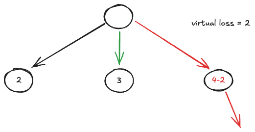
Figure: Virtual loss
Why not just do more parallel games instead of doing virtual loss trick? Typically, an inference server with a GPU is kept ready for model inference which is a bottleneck. To maximize its utilization, it’s important to maintain a steady flow of data using moderately sized evaluation batches. Higher throughput is achieved when fewer parallel games simulated at higher speeds, rather than running many games with only a single simulation thread per game. This way GPU utilisation can be made higher.
Practical Tips
Unit Test in Smaller Environments
To validate the training pipeline early on, I first tested it using a Tic-Tac-Toe environment. This simple baseline is very informative, as it allows you to verify both the MCTS implementation and the training results. MCTS with random rollouts should yield optimal moves from predefined states, and the trained model should learn to reproduce them.
Othello 6x6: The next environment I tackled was Othello on a reduced 6x6 board. It has fewer states than the full game and trains faster, making it a great intermediate testing ground. It’s ideal for iterating on hyperparameters and testing pipeline stability in a more complex setting than Tic-Tac-Toe. Since I am very dumb in this game (tic-tac-toe is about my level of board games), a quick way to test model performance was to pit it against my girlfriend, who is a quite decent player in this game. After the model consistently beat her, I transitioned to the full-board setting. (Only later did I find out that Othello 6x6 is a solved game—but I was too lazy to implement a proper solver-based evaluation.)
Othello 8x8: On the full 8x8 board, training becomes much slower. Here, I benchmark model performance using two key opponents: the Egaroucid bot and a supervised baseline model. One useful early signal that the pipeline is working is the model’s ability to beat MCTS with random rollouts. During the first 7 hours of training, I observed gradual improvement, eventually reaching 100% win rate against this baseline—strong evidence that the pipeline was functioning correctly.
Decide on computational recources
The first instance I used was a Lambda Labs A10G machine with 30 CPUs, which at the end cost me about $100. In the beginning it was attractive for its price and CPU count, but I quickly realized the GPU was underutilized—the model was too small to be bottlenecked by GPU and you do not want to pay for the GPU you are not using.
The real bottleneck was in data collection, which is CPU-bound. I eventually switched to VastAI (not a paid ad, could be though), where I found an RTX 5060 instance with 48 CPUs. For just $18, I trained for a full week. That was enough to reach decent performance with as smaller model and beat Egaroucid at level 7.
Decide on the model size
When compute resources are limited, model size matters. I initially used a supervised learning setup to identify a reasonable model size. Of course, you should first test the pipeline using a small model. Once everything is working, you can do a “YOLO run” with the largest model your budget allows.
Plot stuff
Plot or print as much as possible. Start by observing the agent’s behavior: What moves does it take? How many visits does each node get during MCTS? Are the policy priors aligning with actual visit counts? How does the value function evolve as the game progresses? When and where the value prediction begins to correlate with actual outcomes?
Check signed error: Does the model consistently overestimate or underestimate values? Policy entropy: Has the model collapsed into low-entropy, overconfident decisions too early? MCTS target entropy: If it’s too peaked, you might need more exploration.
Also plot your data distribution: Number of unique states per batch; How conflicting the targets are for the same state; Variance in the value labels for repeated states.
Track how things change over time—this gives you deep insights into training dynamics.
Play with your agent
Test your model in the wild while continuing to monitor metrics. I tested mine extensively using the web version of Egaroucid, which proved far more reliable than testing against other models generated by the same training pipeline. Your models might all share the same bugs or biases, which independent benchmarks help expose.
Explore if the value estimation “jumps” during the game; Were there Unexpected opponent moves that weren’t explored by MCTS and led to losses?
If there was a surprising opponent move, ask:
- Did the policy head ignore this region? → Value head may have been right → decrease c_puct
- Did the value head underestimate it? → Policy was fine → increase c_puct
- Were both wrong? → Worst case → train more
In my experience, err on the side of more exploration. It’s easier to observe meaningful progress when exploration is sufficient. Yes, the model may not be as strong initially, but it’s better to get somewhere first—and only then make it more greedy.
With limited exploration, trajectory variance is low, and training losses may look fine, but real-world performance suffers. This leads you to believe you need a bigger model. But remember: machine learning is a two-sided problem—model and data. The data side usually yields more gains.
Visualizing and improving your data, while keeping the model small for faster iteration, was the strategy that worked for me. Scaling up the model is straightforward next step once the rest is solid.
P.S. You can try playing against the models through a simple UI available here.