Notes on AlphaZero
Recently, I’ve gotten really excited about test-time compute and “Zero” approaches, especially after the release of the O-series models from OpenAI and the DeepSeek-R1-Zero model. Let’s talk about a notable pioneer in this direction: AlphaZero.
I highly recommend reading DeepMind’s AlphaGo Zero paper. To clarify quickly: first verions AlphaGo isn’t a pure “Zero” approach, since it relied on human data to bootstrap, also the pipeline itself is a bit overly complex to read it first. AlphaZero, however, builds directly upon AlphaGo Zero and improves it—essentially maintaining the same pipeline but extending it beyond Go to other games like chess and shogi. Most of the essential technical juice is actually in the AlphaGo Zero paper, so it’s definitely worth checking out first. By the way, I do not think you need more RL knowledge for this paper than what was already discussed in Unconfusing RL: part 1.
AlphaZero represents a crucial step in AI development. It perfectly illustrates the idea behind what’s known as “Sutton’s bitter lesson”, something both David Silver and Richard Sutton emphasize (and that I’m personally a fan of). AlphaZero is a true zero-knowledge approach: it solves problems purely through algorithmic power, computational resources, and environment interactions, without relying on encoded rules or human-crafted knowledge. Basically, it iterates between the two core concepts from Sutton’s essay: search and learning.
This approach has inspired and been extended into many recent developments, most notably the impressive DeepSeek-R1-Zero model. It’s also worth mentioning that David Silver gave a fantastic talk on why reinforcement learning matters, and he has an excellent chapter in a to-be-published book (cannot wait, tbh).
AlphaZero: Intro
AlphaZeroGo is the agent that plays the game of Go. This agent is a neural network that takes as input the current board state (and other useful features like previous states) and outputs the action to take next.
In supervised learning setups, one common approach to create such an agent is to collect expert-level games (played by human professionals or strong computer programs) and train a model to imitate their moves. However, this approach has a main issue: by simply imitating human experts, we’ll never surpass human-level play—because we’re essentially constrained by human knowledge.
Here’s a notable quote from the AlphaGo Zero paper highlighting this point:
“Notably, although supervised learning achieved higher move prediction accuracy, the self-learned player performed much better overall, defeating the human-trained player within the first 24 hours of training. This suggests that AlphaGo Zero may be learning a strategy that is qualitatively different from human play.”
Another intuitive approach could be trial-and-error learning, since we have access to the Go environment through a simulator. However, Go requires an opponent to play against, and ideally, this opponent should always match your skill level: not too easy, not too hard. If your opponent is too easy, you won’t learn much—you’ll just dominate every game. If your opponent is too strong, you’ll continually lose, resulting in overwhelming negative feedback and limited learning progress. Interestingly, this “too-strong-opponent” issue isn’t actually a significant problem in AlphaZero’s case—challenging opponents can actually accelerate learning significantly. But since we’re adopting a pure “Zero” approach, we have no external opponent at all. The elegant solution: self-play. You just play against yourself repeatedly. Add in a grain (well, actually a bit more than that) of exploration, and during these countless matches, you’ll stumble across innovative strategies and useful moves to reinforce in your training. Without exploration the learning process may stuck into local, non-optimal solutions.
Finally, there’s one crucial question remaining: how exactly do we handle exploration, and how do we reinforce good moves? Could we just sprinkle some epsilon-noise and apply a basic policy-gradient algorithm like REINFORCE, and then call it a day? Call me crazy, but I bet you need a better exporation strategy due to the astronomical size of Go’s state-space: approximately \(10^{170}\) legal board positions (for comparison, chess has about \(10^{47}\)—still huge). Random exploration alone won’t cut it. To address this, AlphaZero suggests leveraging Monte Carlo Tree Search (MCTS). MCTS helps with intelligent planning by selectively exploring promising moves in a tree structure, focusing computational resources on the most relevant parts of the search space. This provides richer, higher-quality supervision signals for our policy neural network. After each self-play game guided by MCTS, we use supervised learning to update the network. Then, repeat.
Why can’t we rely on plain actor–critic (or REINFORCE)? The chance of stumbling on an informative but low-prior move is astronomically small. Even if the policy does discover a good move, the signal from the final reward is far too weak. When you make a single random move, you only find out whether it was good or bad at the end of the game. If, instead, you run hundreds of simulations from the same position—trying many continuations—and return a full visit-count distribution plus a bootstrapped value, you provide a much richer learning target.
Why doesn’t every discrete RL problem adopt MCTS?
Two prerequisites make MCTS hard to apply widely:
- You need to have a model of the environment.
You either have it like in board games or you learn it (checkout MuZero) - the last is a challenging step on its own.- The environment should near-deterministic.
Stochastic dynamics explode the tree and simulation becomes infeasible to get any low-variance signal. Check out interesting work on Sampled MuZero for huge action spaces and determenistic environments.
AlphaZero: Algorithm
To grasp the main idea behind AlphaZero, we primarily need diagram below from the original paper. The figure depicts the action-selection process from a given game state, which is used both during self-play data collection (training) and inference (actual gameplay). At the core, we have a neural network that takes the current state \(s\) and outputs two things:
- Policy distribution \(p(s)\), indicating probabilities for possible next moves.
- Value estimate \(v(s)\), predicting how good the current position is.
Initially, this neural network’s weights are random, but they improve iteratively through training.
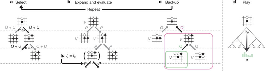
Figure: AlphaGoZero
Let’s carefully walk through how exactly we collect a training set.
1. Training Dataset Collection:
We simulate a self-play game, and for each state encountered during the game, we perform the following steps:
a. Select (Exploration Phase)
-
A simulation starts from the given state \( s \).
-
Moves are chosen greedily to maximize a combination of exploitation (value estimate \( Q(s, a) \)) and exploration (bonus \( U(s, a) \)):
\[ a_t = \arg\max_a \left[ Q(s, a) + U(s, a) \right] \]
-
This approach ensures balanced exploration of new actions and exploitation of known good actions.
-
The search continues until a leaf node (an unexpanded node) is reached.
Value estimate:
\[ Q(s, a) = \frac{W(s, a)}{N(s, a)} \]
Where: \( W(s, a) \) is the cumulative value from simulations starting from action \( a \) in state \( s \), and \( N(s, a) \) is the visit count for action \( a \) in state \( s \).
Exploration bonus:
\[ U(s, a) = c_{puct} \cdot P(s, a) \cdot \frac{\sqrt{\sum_b N(s, b)}}{1 + N(s, a)} \]
Where: \( P(s, a) \) is the prior probability of action \( a \), provided by the neural network policy \( p(s) \), and \( c_{puct} \) is a constant controlling the trade-off between exploration and exploitation.
b. Expand and Evaluate
-
When reaching a leaf node \( s_L \), evaluate it with the neural network to obtain: \( (p(s_L), v(s_L)) \) - prior distribution for the next moves and value of this leaf state
-
If the node represents a terminal state (i.e. end of the game), assign the true reward from the environment as the value.
-
If it's not terminal, expand the node by initializing its children’s priors using the neural network policy \( p(s_L) \). Higher priors mean that the node will be explored more frequently during future simulations.
AlphaGo vs. AlphaZero: AlphaGo employs Monte Carlo rollouts (random simulations from the leaf node) to estimate leaf-node values, making it a traditional MCTS method with unbiased but high-variance estimates. In contrast, AlphaGo Zero (and AlphaZero) eliminate rollouts entirely, relying solely on neural network predictions of leaf-node values \( v(s_L) \), learned from self-play. This resembles a Temporal Difference (TD) method: biased but lower-variance due to bootstrapping on the current value function.
c. Backup
-
After evaluation, propagate the obtained value \( v(s_L) \) back up the tree.
-
For each node along the path from the leaf node \( s_L \) back to the root \( s_0 \), update its cumulative statistics:
-
Increment visit count:
\[ N(s, a) \leftarrow N(s, a) + 1 \]
-
Update cumulative value:
\[ W(s, a) \leftarrow W(s, a) + v(s_L) \]
-
-
This step effectively reinforces promising paths and reduces confidence in weaker ones. This averaging process improves the decisions over time, and makes MCTS to choose better actions.
d. Play (Action Selection)
-
Once enough simulations have been performed, play an actual move based on the visit counts of the root node’s children.
-
Specifically, compute a probability distribution over actions using the visit counts:
\[ \pi(a \mid s) = \frac{N(s, a)^{1/\tau}}{\sum_b N(s, b)^{1/\tau}} \]
-
Where:
\( \tau \) is a temperature parameter that controls exploration.
Typically, \( \tau \) is:
- High early in self-play games (to encourage exploration).
- Low or near 0 later in the game (to become greedy and decisive) or during inference.
-
Sample the next action \( a \) from the distribution \( \pi(a \mid s) \).
-
Record the resulting policy vector \( \pi(a \mid s) \) as the training target for the policy head of the neural network.
Repeat the above steps until the game ends:
- At the end of a self-play game, the final outcome (win/loss/draw) is known. This outcome becomes the ground truth value for each state encountered during the game: each state \(s_t\) is assigned a ground truth value based on the final game outcome from the perspective of the current player at that state.
-
We have a training dataset of triples:
\[\{(s_1, \pi_1, z), (s_2, \pi_2, z), \dots, (s_T, \pi_T, z)\}\]where:
- \(s_t\) is a state visited during the game,
- \(\pi_t\) is the policy (visit-count-based) distribution,
- \(z \in \{-1, 0, 1\}\) is the final game outcome from the perspective of the current player at state \(s_t\).
Let’s do it a couple (or a thousand) more times, and you’ve got yourself a training set for your model that you can store in the replay buffer.
- Why UCB-style exploration is chosen?
- Are there scenarios where Tomposon sampling would be better?
2. Model Training:
Given the replay buffer filled with samples collected from the previous step (and from earlier steps), we train the neural network using supervised learning. Specifically, the model is trained by minimizing the following combined loss:
\[\mathcal{L} = (z - v)^2 - \pi^\top \log p + c \|\theta\|^2\]where:
- MSE loss between \(z\) - the true outcome of the game from the perspective of the player at state \(s\) and \(v\) - the predicted value output of the network for state \(s\).
- Cross-entropy loss between \(\pi\) - the MCTS policy distribution (visit-count-based probabilities from the self-play phase) and \(p\) - the predicted policy output by the neural network for state \(s\).
- \(c \|\theta\|^2\) is an optional L2 regularization term used to prevent overfitting.
Compute the loss, compute the gradient, update the model, you know the drill. Then, return to step 1 to collect more data with the improved policy. This closes the Reinforcement Learning loop.
Value and Policy Models: At the end of training, both the policy and value networks are quite powerful on their own. You can use the policy model to directly predict the next move, or the value model to evaluate potential next states and choose the one with the highest predicted value. However, combining both in practice yields significantly better performance than either model used in isolation.
Why? As far as I understand, these etimates balance the error profiles of each other. The value estimate is high-variance, but low-bias - it can recognise long-term advantages (deep tactics). The policy estimate is high-bias, but low-variance - it reliably proposes locally strong moves, but may overlook deep tactical lines. By balancing both we try to achieve a better overall trade-off.
Model Promotion in AlphaGo Zero vs. AlphaZero
There is one more step after training in AlphaGoZero: model promotion. This step is one of the main differences between AlphaGoZero and AlphaZero:
-
AlphaGoZero employs an explicit evaluation step:
- Two models are maintained: the current training model and the best-performing model so far.
- After each training iteration, the current model is evaluated against the best model by playing a set of evaluation games.
- If the current model performs significantly better (e.g., wins the majority of games), it replaces the best model.
- This new best model is then used for self-play in future cycles.
- While this evaluation adds stability, it slows down training due to delayed promotion.
-
AlphaZero simplifies this process:
- There is no explicit evaluation phase between models.
- The latest trained model is always used to generate self-play data.
- This allows for faster convergence, though it can sometimes introduce instability or short-term performance regressions.
- Does the AlphaZero loss remind us actor-critic loss? What is different?
AlphaZero: Policy Iteration
Now, let’s briefly reflect on the algorithm discussed in the previous section. The AlphaZero training loop can be summarized in the following steps:
1. Start with a neural network that outputs a policy vector and a value scalar for any given game state.
2. Use it inside MCTS, which:
– explores the search tree using the network outputs,
– returns an improved policy vector (search probabilities),
– selects a move,
– and records this policy vector in a buffer.
3. Repeat until the end of the game and record the final reward (game outcome).
4. Train the model:
– distill the improved policy into the model,
– make it predict the true final reward for each state.
5. Go back to step 1.
The key insight here is that each iteration yields a neural network that produces better predictions, enabling the subsequent MCTS simulations to further refine the policy. Essentially, this loop is an instance of generalized policy iteration (GPI), where Monte Carlo Tree Search simultaneously performs policy evaluation and policy improvement steps:
-
Policy Evaluation:
MCTS evaluates states by running simulations guided by the neural network’s current predictions. This results in more accurate state-value estimates and action probabilities than the raw outputs from the neural network alone. -
Policy Improvement:
During simulations, MCTS uses the Upper Confidence bound criterion, which progressively focuses on moves with potentially higher payoffs. By returning the normalized visit counts as an “improved” policy vector, MCTS explicitly performs the policy improvement step. Later, we distill this improved policy back into the neural network via supervised learning.
AlphaZero: Can we solve the game?
Does this generalized policy improvement loop guarantee convergence to the optimal policy? Can we essentially “solve” games like Chess or Go if we wait long enough?
Consider board games like Chess or Go, which can be modeled as finite-state Markov Decision Processes (MDPs)—though with enormous state spaces. Classical reinforcement learning theory provides strong theoretical guarantees: for finite-state MDPs with tabular representations and sufficient exploration, methods like Monte Carlo or Temporal Difference (TD) learning indeed converge to optimal solutions. This theoretical guarantee would under strict conditions:
- Tabular representations for both value and policy functions (storing exact values for every state individually).
- Sufficient exploration (visiting all relevant states infinitely often).
Thus, in theory, with explicit tabular representations and unlimited computational resources, Chess or Go could indeed be “solved,” as methods like Policy Iteration and Value Iteration are guaranteed to converge to the optimal policy/value.
However, this scenario is entirely impractical due to the sheer size of the state space (approximately \(10^{47}\) for Chess and \(10^{170}\) for Go), making tabular methods computationally infeasible. Moreover, pure Monte Carlo Tree Search (without function approximation) can’t generalize information between similar states—each state is treated independently, further limiting its practical effectiveness. AlphaZero addresses this problem by employing function approximation (specifically, neural networks). Instead of storing exact values and policies for every state, AlphaZero generalizes across states, using learned representations to approximate both policy and value functions. This generalization improves efficiency by allowing experience gained from one state to benefit similar states.
AlphaZero is known to be approximate policy iteration with neural network function approximation. In this case leaf node values are not exact terminal rewards but approximations: hence there are approximation errors. Classical theory assumes sufficient exploration and exact (tabular) state-value representation. AlphaZero breaks this theoretical assumptions. Thus, we lose absolute theoretical guarantees of convergence to global optimum.
AlphaZero: Can we stuck in local optimum?
When applying evaluation and improvement operators, our goal is essentially to find a fixed point for our parameters. Although this fixed point ideally represents the global optimum, it’s possible to get stuck in local optima, potentially leading to degenerate strategies.
There are important points to clarify beforehand. When using Monte Carlo Tree Search (MCTS) combined with the Upper Confidence Bound applied to Trees (UCT) algorithm for guiding the search, it is proven that the probability of selecting the optimal action converges to 1 as the number of samples grows to infinity. Therefore, with an infinite simulation budget, MCTS with UCT can theoretically solve the game. Notice that in this setting, value estimation is purely Monte Carlo-based and unbiased; we do not rely on any neural approximations. Instead, the values for each move must be explicitly stored in a table.
The UCT formula is given by:
\[UCT(s, a) = V_{MC}(s, a) + c \cdot \sqrt{\frac{\ln{N(s)}}{N(s, a)}}\]In contrast, AlphaZero employs a different formula called PUCT (I guess there is a better option), which incorporates learned neural network priors for action selection within MCTS:
\[PUCT(s, a) = V_{\theta}(s, a) + c \cdot P_{\theta}(s, a) \cdot \frac{\sqrt{N(s)}}{1 + N(s, a)}\]This neural-guided search significantly improves efficiency by biasing simulations toward promising moves. However, the inclusion of a learned prior means that PUCT does not strictly inherit UCT’s convergence guarantee. By using a neural network, we introduce bias into the search process. Policy: Suggests likely promising moves (reducing branching factor). Value: Provides quick, approximate assessments of positions (reducing depth needed). Consequently, a poorly trained or misguided prior could negatively influence exploration. For instance, if the network erroneously assigns a near-zero prior probability to the genuinely optimal move, the PUCT exploration term might neglect that move entirely, effectively ignoring potentially optimal moves. To counteract this potential failure mode, AlphaZero mitigates the issue by adding small Dirichlet noise to the prior at the root of each self-play game. This ad-hoc exploration ensures occasional exploration of every legal move, preventing complete neglect of any potentially good action.
Essentially, to maintain theoretical convergence guarantees, one must use the UCT formula for exploration in MCTS. This would imply performing many unbiased rollouts until the end of the game to estimate leaf values combined with a uniform prior for selecting moves within the tree search.
What does happen if AlphaZero got stuck? I guess MCTS produces essentially identical move distributions as the neural policy and Neural network no longer improving significantly between iterations. In such a scenario, it likely means there isn’t enough exploration and MCTS cannot pull the network from this local optima, causing the training process to stall. A concrete example of this failure mode was highlighted in a paper (see here), which stated:
“AlphaZero can fail to improve its policy network if it does not visit all actions at the root of the search tree.”
In other words, if the MCTS guided by the current network never tries a potentially strong move, then that move will never be selected in self-play, and the network will never learn its value.
AlphaZero: on/off-policy
Is AlphaZero an on-policy or an off-policy algorithm?
-
If we define the policy strictly as the combination of MCTS + neural network, then the policy we use for generating data (behavioral policy) and the policy we’re improving (target policy) are identical. This aligns AlphaZero more closely with on-policy learning.
-
However, AlphaZero’s practical implementation includes a replay buffer containing previously generated self-play games. These games were collected using slightly different (older) versions of the neural network—meaning that the behavior policy used to collect the data differs from the current network being updated.
This detail technically makes AlphaZero an off-policy algorithm. The larger the replay buffer (and the older the stored games), the more off-policy the updates become. This introduces drawbacks:
-
Slower convergence: The neural network is updated using trajectories generated from older policies, potentially less relevant to the current policy. This mismatch can slow down learning since the network tries to approximate policies that are no longer optimal or even relevant. For instance, the current agent might convert that same position into a win, yet it is trained on a label that says “draw,” planting systematic bias.
-
Potential instability: Excessively off-policy training can lead to training instability or oscillations, as the network must adapt to policy differences accumulated over many iterations.
On the other hand, maintaining a replay buffer with historical trajectories has important benefits:
-
Prevents catastrophic forgetting: Showing older trajectories during training helps the model retain previously learned strategies and avoid drifting into overly narrow or suboptimal solutions.
-
Improves sample efficiency: Reusing past experiences ensures the network doesn’t forget robust strategies learned earlier.
Trade-off, the usual stuff.
The remarkable practical success of AlphaZero is well captured by the following quote from the AlphaGo Zero paper:
“Humankind has accumulated Go knowledge from millions of games played over thousands of years, collectively distilled into patterns, proverbs, and books. In the space of a few days, starting tabula rasa, AlphaGo Zero was able to rediscover much of this Go knowledge, as well as novel strategies that provide new insights into the oldest of games.”