Unconfusing RL: part 1. MDP
In this series of notes, titled Unconfusing RL, I aim to summarize what I consider the essential concepts of Reinforcement Learning (RL). This is my personal attempt to deepen my understanding, draw connections between algorithms, share insights with others, and create a central repository of comprehensive notes on RL that I can return to. I hope someone will benefit from it as well.
Why This Series? Reinforcement Learning can often feel intimidating and difficult to grasp. While excellent books and courses exist, I’ve found that even after studying the same algorithms and concepts multiple times, things can remain unclear—at least, that has been my experience. Sometimes, to truly understand something, we need to slow down, revisit the basics, and ask deeper questions. I will try to do that in this series of notes.
Disclaimer: Please note that these notes are more like “filling-the-gaps” materials rather than self-contained articles or lectures. For instance, I might skip over well-known definitions or properties unless they are critical for understanding the discussion. This will help to keep it concise and avoid creating yet another article on things like (MDP, Q-learning, *Put your banger*) explained.
What is this note about?
In this note, I’ll reflect on the Markov Decision Process (MDP)—why it’s a core component of RL, the significance of understanding the dynamics of the environment (i.e., knowing the MDP), and how this knowledge influences algorithm design.
Why MDP?
Whenever we have a decision-making process, we need a way to model it. An MDP is a mathematical framework that helps in modeling situations where the outcomes of decisions are partly random and partly under the control of a decision-maker. RL deals with sequences of such decisions. Even when the outcomes of actions are deterministic, the MDP framework still applies—deterministic outcomes can be represented using a Dirac delta function as the probability density. Our decision-maker (an agent) needs to come up with a plan for every possible state. This plan is a policy, and it is usually stochastic when the agent returns a probability distribution over actions.
MDPs assume the environment satisfies the Markov property, where the current state contains all the necessary information to make the next decision. Notice that the transition probability matrix fully characterizes the environment’s dynamics. This means that if you know this matrix (along with the set of states, actions, and rewards), you know everything about MDP. Notice that many real-world problems do not possess a Markov property, usually, it is only an approximation. Here is an interesting fact: Recurrent Neural Networks can be used to keep the compression of the history in the hidden variable which helps to bring the problem closer to satisfying Markov property.
Why Is MDP a convenient framework?
- MDPs are easy enough to derive a theoretical foundation for reinforcement learning problems.
- Many problems can be framed as an MDP. For example, the Atari Pong game with one frame as a state is not an MDP because the state doesn’t encode the direction of the ball. However, if a state includes four consecutive frames, it becomes an MDP, as the sequence provides enough information to determine the ball’s direction.
Bellman equation
In RL, we aim to maximize a scalar quantity called the reward. A reward, denoted as \(R\), is associated with any transition taken within the MDP of the environment. The cumulative reward over a trajectory is denoted as \(G\), which is typically discounted using a constant \(\gamma \in [0, 1]\). This cumulative reward is a sample, and our goal is to maximize the expectation over these samples, \(\mathbb{E} \left[G\right]\). To be able to compare policies we need to have some metric which correlates with \(\mathbb{E} \left[G\right]\). The value function and action-value function serve as these metrics, helping us evaluate and optimize policies.
The value function \(V_\pi(s)\) represents the expected cumulative reward starting from a given state \(s\) and following a specific policy \(\pi\):
\[V_{\pi}(s) = \mathbb{E}_{a \sim \pi, s_{t + 1} \sim P} \left[ G_t \mid S_t = s \right] = \mathbb{E}_{a \sim \pi, s_{t + 1} \sim P} \left[ R_{t+1} + \gamma V_{\pi}(S_{t+1}) \mid S_t = s \right]\]The subscript \(\pi\) in the value function indicates that the expectation depends on the policy (i.e., the action \(a\) chosen). If you behave differently (follow a different policy), you will receive a different reward. The above equation is called the Bellman Expectation Equation. For a formal proof of why the value function for the next state can be written under the expectation sign, refer to this explanation.
Similarly, for the action-value function \(Q_\pi(s, a)\), which measures the expected cumulative reward starting from state \(s\), taking action \(a\), and then following policy \(\pi\), we have:
\[Q_{\pi}(s, a) = \mathbb{E}\left[ G_t \mid S_t = s, A_t = a \right] = \mathbb{E}\left[ R_{t+1} + \gamma Q_{\pi}(S_{t+1}, A_{t + 1}) \mid S_t = s, A_t =a \right]\]Let’s discuss a more detailed derivation of the Bellman Expectation equation by analyzing the decision-making process illustrated below. First, given a state \(s\), we choose an action according to some policy \(\pi\): \(a \sim \pi\). This leads to the following equation for the value function:
\[V_{\pi}(s) = \sum_a \pi(a|s) Q_{\pi}(s, a)\]
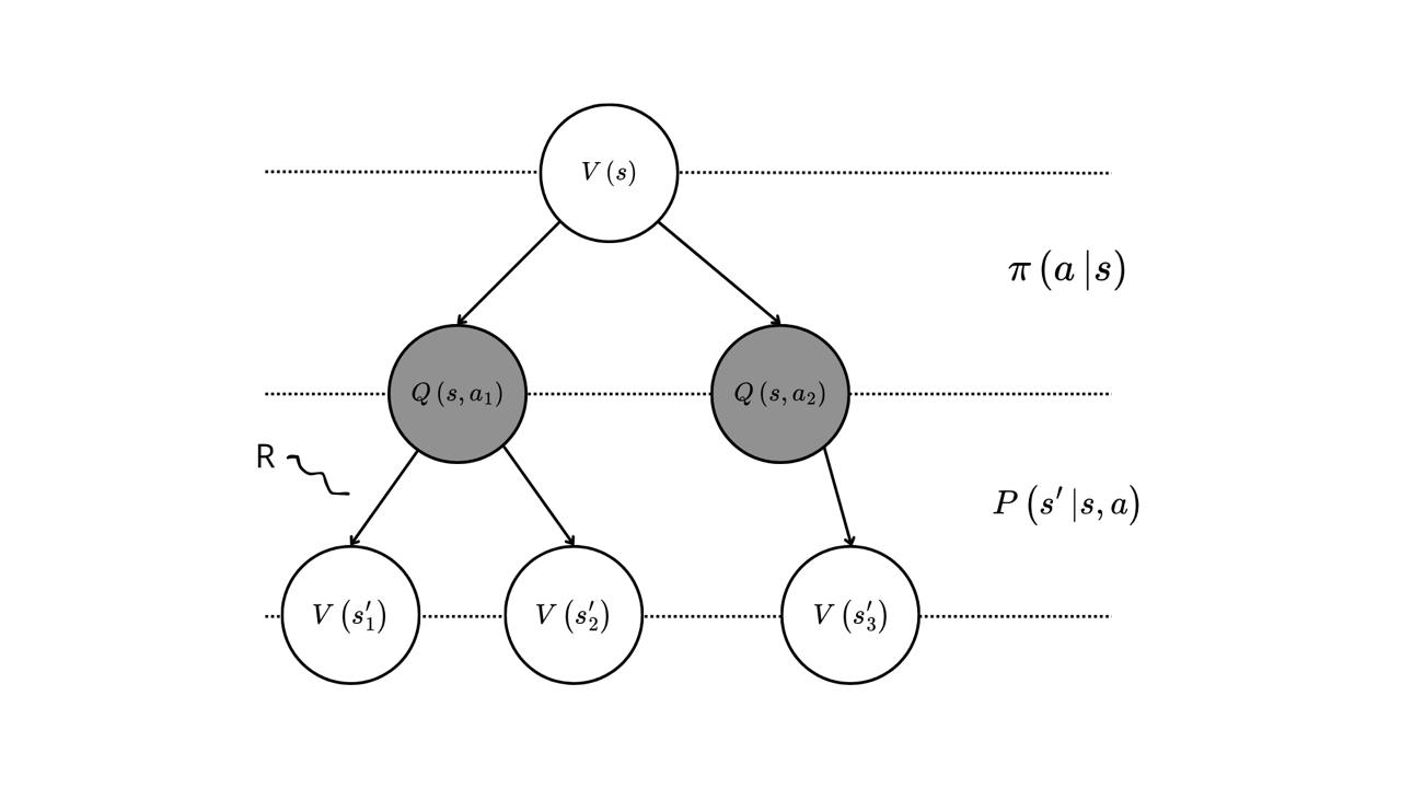
Figure: MDP graph
Next, given an action \(a\) and the starting state \(s\), the environment reacts by transitioning to the next state \(s'\) according to the transition probability distribution \(\mathbb{P}(s' \mid s, a)\). A reward \(R(s, a, s')\) is also obtained during this transition. This results in the following equation for the action-value function:
\[Q_{\pi}(s, a) = \sum_{s'} \mathbb{P}(s' \mid s, a) \left[ R(s, a, s') + \gamma V_{\pi}(s') \right]\]Finally, by combining the above equations, we arrive at:
\[V_{\pi}(s) = \sum_a \pi(a|s) \sum_{s'} \mathbb{P}(s' \mid s, a) \left[ R(s, a, s') + \gamma V_{\pi}(s') \right]\]The Bellman Expectation Equation describes the estimation problem of a value function for a given policy. The Bellman Optimality Equation (first equal sign below), on the other hand, describes the problem of finding the optimal policy by determining the optimal value function. It assumes that the policy is greedy, meaning that we select actions based on the best action-value function. This leads to the following equation:
\[V_{*}(s) = \max_a Q_{*}(s, a) = \max_a \sum_{s'} \mathbb{P}(s' \mid s, a) \left[ R(s, a, s') + \gamma V_{*}(s') \right]\]On Q-function and V-function practical difference: If you have the optimal value function \(V_{*}\), you could use the MDP to do a one-step search for the optimal action-function \(Q_{*}\) and then use this to build the optimal policy. On the other hand, if you had the \(Q_{*}\), you don’t need the MDP at all. You could use the optimal \(Q_{*}\) to find the optimal \(V_{*}\) by merely taking the maximum over the actions: \(V_{*}(s) = \max_a Q_{*}(s, a)\). Similarly, you could obtain the optimal policy \(\pi_{*}\) using the optimal \(Q_{*}\) by taking the argmax over the actions. This implies that if the MDP of your environment is unknown (as is often the case), knowing the \(V_{*}\) alone is insufficient to derive the policy (we cannot do a one-step search since probabillities of the transitions are unknown). Instead, estimating the \(Q_{*}\) directly (as done in algorithms like Deep Q-Networks (DQN)) is more practical.
The Bellman Expectation Equation is a linear equation in terms of the value function. Hence, given the MDP dynamics (i.e., the transition probabilities and rewards are known), one can solve it directly using a closed-form solution. The Bellman Optimality Equation is a non-linear equation due to the max operation over actions. In general, there is no closed-form solution for this equation, but it has a unique solution because of the contraction property of the Bellman operator (discussed below). Since no closed-form solution exists, iterative methods are required to solve it.
For the Bellman Expectation Equation, we can rewrite it in matrix form. Let \(\mathbf{R}^\pi\) represent the expected reward vector for a given policy \(\pi\), and \(\mathbf{P}^\pi\) represent the state transition probability matrix under the policy. The equation is given by:
\[\mathbf{V}_{\pi} = \mathbf{R}^\pi + \gamma \mathbf{P}^\pi \mathbf{V}_{\pi}\]Solving for \(\mathbf{V}_{\pi}\), we get:
\[\mathbf{V}_{\pi} = (\mathbf{I} - \gamma \mathbf{P}^\pi)^{-1}\mathbf{R}^\pi\]Where:
- \(\mathbf{I}\) is the identity matrix.
- \(P^\pi_{ij} = \sum_a \pi(a \mid s_i) P(s_j \mid s_i, a)\), which defines the probability of transitioning from state \(s_i\) to state \(s_j\) under policy \(\pi\).
The matrix \((\mathbf{I} - \gamma \mathbf{P}^\pi)\) is invertible because \(\gamma < 1\) and \(\mathbf{P}^\pi\) is a stochastic matrix (its rows sum to 1). The solution to the Bellman Expectation Equation is therefore unique, and it can be computed directly with a computational complexity of \(O(n^3)\), where \(n\) is the number of states. However, this approach becomes computationally expensive when the number of states is very large. In such cases, it is more practical to use iterative methods, which are computationally efficient and scalable. As we will discuss below, both the Bellman Expectation Equation and Bellman Optimality Equation can be solved using Dynamic Programming (DP) techniques.
A take on exploration/exploitation: In real-world examples, the MDP usually is not known. You may not know the probability of outcomes and even the set of outcomes itself. So, in these cases one needs to explore, this will help to estimate what outcomes with what probability could occur. When an agent has full access to an MDP, one can calculate the expectations directly by just looking at the dynamics probabilities and rewards, given that this calculation is feasible (you may know the MDP, but it can be too huge to be practically used in other ways but in a sampled-based manner, e.g. chess, go). In this case, there is no need for exploration! The policy/value iteration methods described below are examples of dynamic programming methods where MDP is assumed to be known. Hence there is no need to interact with the environment and no trial-and-error learning.
Dynamic programming
Remember solving Dynamic Programming (DP) problems during coding interviews? Is it any different from the DP we discussed above in the context RL? Not really. DP, in both contexts, involves iterative methods that share a common structure:
- The problem can be decomposed into smaller subproblems.
- Solutions to subproblems can be saved and reused to solve larger problems efficiently.
For instance, here is the solution to the LeetCode Coin Change Problem using a value iteration-like approach. Two well-known DP methods to find an optimal policy are: Policy iteration and Value iteration.
Policy iteration
Policy iteration consists of two main steps:
- Policy Evaluation: Evaluate how good a given policy is by calculating its value function.
- Policy Improvement: Use the results from policy evaluation to create a new, improved policy by acting greedily with respect to the value function.
The ability to evaluate your decisions is critical in any optimization process. Once you have a reliable evaluation, optimizing becomes more straightforward. Policy iteration embodies this principle:
- Start with an initial policy and a given MDP.
- Evaluate its performance by computing the value function.
- Improve the policy using a greedy approach.
- Repeat until the policy no longer changes.
Below is a scheme that illustrates this process. Taken from this article.
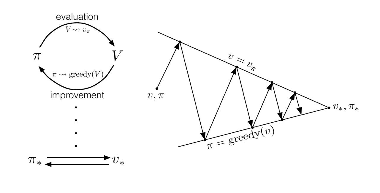
Figure: Generalized Policy Iteration.
The policy improvement converges when it is greedy with respect to the current value function. The value function evaluation converges when it is consistent with the current policies. Each process messes up the consistency of another process, but both of them eventually converge to the fixed point. In a sense, they work towards a common goal, as depicted in the right plot of the above figure.
Policy Evaluation: take the Bellman Expectation equation and convert it to the iterative update. The process of estimating the value function for the given policy is iterative and proven to converge given that the Bellman operator is a contraction.
\[v_{k+1}(s) = \sum_a \pi(a|s) \sum_{s'} \mathbb{P} (s' | s, a) \left[ R(s, a, s') + \gamma v_{k}(s') \right]\] def policy_evaluation(env, policy: np.array, gamma: float) -> np.array:
""""Estimation of the value function"""
theta = 1e-6
prev_Q = np.zeros((env.observation_space.n, env.action_space.n))
MDP = env.unwrapped.P
while True:
# Bellman operator is a contraction
# Iterate long enough -> Convergence
Q = np.zeros((env.observation_space.n, env.action_space.n))
for s in range(env.observation_space.n):
for a in range(env.action_space.n):
# Compute the Q-value for (state, action) pair
# iterate over all possible outcomes from the (state, action)
# for the next Q iterate over actions
Q[s][a] = sum(
prob * (reward + gamma * (not done) *
sum(policy[next_state][next_action] *
prev_Q[next_state][next_action]
for next_action in range(env.action_space.n)))
for prob, next_state, reward, done in MDP[s][a])
# Check for convergence
if np.max(np.abs(prev_Q - Q)) < theta:
break
prev_Q = Q.copy()
return prev_Q
Policy Improvement: imagine you have an existing policy and are considering changing it. How can you determine if the new policy is better? To evaluate this, you can compare the value function of the current state \(V_{\pi'}(s)\) under the new action to the action-value function of the old policy \(Q_{\pi}(s, \pi(s))\). Specifically, if in a given state you choose a different action and then follow your old policy, you can compare the resulting values. If you choose actions greedily in a given state, it can be shown that you are at least not doing worse for any state:
\[V_{\pi'}(s) \ge Q_{\pi}(s, \pi'(s)) = \max_a Q_{\pi}(s, a) \ge Q_{\pi}(s, \pi(s)) = V_{\pi}(s), \forall s\]A natural extension of this idea is to choose greedy actions in all states. This leads to the principle that a greedy policy, based on the action-value function, improves the policy. If there is no further improvement, we reach the Bellman Optimality Equation, and the policy becomes optimal:
\[\max_a Q_{\pi}(s, a) = Q_{\pi}(s, \pi(s)) = V_{\pi}(s) \implies V_{\pi}(s) = V_{*}(s), \forall s\]This means that we have a method to improve the policy which is proven to converge to the optimal policy. First, we evaluate the action-value function for all states, then we take greedy action for each state, then repeat.
This means that we have a systematic method to improve the policy, which is guaranteed to converge to the optimal policy. The process involves:
- Evaluating the action-value function \(Q_{\pi}(s, a)\) for all states.
- Taking greedy actions for each state based on the current action-value function.
- Repeating the process until no further improvements can be made.
One could see that these reminds expectation–maximization algorithms.
- The policy evaluation step corresponds to the “Expectation” step, where we estimate the value function (or action-value function) under the current policy.
- The policy improvement step corresponds to the “Maximization” step, where we refine the policy by choosing greedy actions.
  def greedify(Q):
      """Greedify policy: policy improvement"""
      new_pi = np.zeros_like(Q)
      new_pi[np.arange(Q.shape[0]), np.argmax(Q, axis=1)] = 1
      return new_pi


  def policy_iteration(env, policy, gamma=0.9, theta=1e-6):
      """Policy iteration"""
      while True:
          old_policy = policy.copy()
          Q = policy_evaluation(env, policy, gamma)
          policy = greedify(Q)
          if np.max(np.abs(old_policy - policy)) < theta:
              break

      return policy, Q
- Is policy iteration applicable to non-tabular settings?
- Does SARSA have anything to do with the policy iteration?
Value iteration
Take the Bellman Optimality equation and convert it to the iterative update, this forms the basis of the Value Iteration Algorithm. It is a one-step lookahead algorithm based on the idea that we already know the optimal value function \(v^*\) for the next step. The update rule is as follows:
\[v_{k+1}(s) = \max_a \sum_{s'} \mathbb{P}(s' \mid s, a) \left[ R(s, a, s') + \gamma v_k(s') \right]\]Unlike Policy Iteration, where the value function corresponds to the value of a specific intermediate policy at every step, the intermediate value functions in Value Iteration do not necessarily correspond to any real policy. Instead, they are approximations converging toward the optimal value function \(v^*\).
Optimal Policy Extraction: once \(v^*\) is obtained, the optimal policy \(\pi^*\) can be derived by acting greedily with respect to \(v^*\):
\[\pi^*(s) = \text{argmax}_a \sum_{s'} \mathbb{P}(s' \mid s, a) \left[ R(s, a, s') + \gamma v^*(s') \right]\]Value Iteration can be seen as a special case of Generalized Policy Iteration (GPI), where the “policy improvement” step is deferred until the value function has fully converged.
- Does Q-Learning have anything to do with the value iteration?
Why does Policy / Value iteration converge?
The Bellman Expectation Operator is defined as:
\[\mathbf{T}^\pi (\mathbf{V}) = \mathbf{R}^\pi + \gamma \mathbf{P}^\pi \mathbf{V}\]where:
\[\mathbf{R}^\pi = \sum_a \pi(a \mid s) \sum_{s'} \mathbb{P}(s' \mid s, a) R(s, a, s')\] \[\mathbf{P}^\pi_{ij} = \sum_a \pi(a \mid s_i) \mathbb{P}(s_j \mid s_i, a)\]The Bellman Optimality Operator is defined as:
\[\mathbf{T}^* (\mathbf{V}) = \max_a \left[\mathbf{R}^a + \gamma \mathbf{P}^a \mathbf{V}\right]\]where:
\[\mathbf{R}^a = \sum_{s'} \mathbb{P}(s' \mid s, a) R(s, a, s')\] \[\mathbf{P}^a_{ij} = \mathbb{P}(s_j \mid s_i, a)\]Both operators are contractions, this guarantees that repeated applications of the operator \(\mathbf{T}\) reduce the distance between successive value function estimates, ensuring convergence. They have a unique fixed point, this means that convergence happens to a unique point by iteratively applying these operators.
- For the Bellman expectation operator \(\mathbf{T}^\pi\), the unique fixed point is the value function of the policy \(V^\pi\), (proof). Policy Evaluation converges to \(V^\pi\) under \(\mathbf{T}^\pi\).
- For the Bellman optimality operator \(\mathbf{T}^*\), the unique fixed point is the optimal value function \(V^*\), which satisfies the Bellman Optimality Equation. Value Iteration converges to \(V^*\) under \(\mathbf{T}^*\).
Wrapping up
Here, we considered the case when the MDP is fully known. In computationally feasible scenarios, this knowledge does not require us to interact with the environment or do any trial-and-error learning. This represents the best-case scenario. However, in most real-world problems, the MDP of the environment is not known. In such cases, we will need to explore the environment, which introduces additional complexity. This will require the use of sample-based algorithms, such as SARSA and Q-Learning, to estimate the dynamics and rewards of the environment and ultimately find an optimal policy. Stay tuned!
Used Resources
- UCL Course by David Silver
- Reinforcement Learning: An Introduction by Richard S. Sutton and Andrew G. Barto
- Grokking Deep Reinforcement Learning by Miguel Morales
- Coding example using value iteration and policy iteration to solve the FrozenLake-v1 environment.